Functional Data Analysis

Key Learning Outcomes

---

After completing this module the trainee should be able to:

• Understand how EMG provides functional analysis of metagenomic data sets

• Know where to find and how to interpret analysis results for samples on the EMG website

• Know how to download the raw sample data and analysis results for use with 3^rd party visualisation and statistical analysis packages

Resources You’ll be Using

---

Tools Used

Megan6 : http://ab.inf.uni-tuebingen.de/software/megan6/

Useful Links

---

EBI Metagenomics resource (EMG) :
www.ebi.ac.uk/metagenomics/

Introduction

---

The EBI Metagenomics resource (EMG) provides functional analysis of predicted coding sequences (pCDS) from metagenomic data sets using the InterPro database. InterPro is a sequence analysis resource that predicts protein family membership, along with the presence of important domains and sites. It does this by combining predictive models known as protein signatures from a number of different databases into a single searchable resource. InterPro curators manually integrate the different signatures, providing names and descriptive abstracts and, whenever possible, adding Gene Ontology (GO) terms. Links are also provided to pathway databases, such as KEGG, MetaCyc and Reactome, and to structural resources, such as SCOP, CATH and PDB.

What are protein signatures?

Protein signatures are obtained by modelling the conservation of amino acids at specific positions within a group of related proteins (i.e., a protein family), or within the domains/sites shared by a group of proteins. InterPro’s different member databases use different computational methods to produce protein signatures, and they each have their own particular focus of interest: structural and/or functional domains, protein families, or protein features, such as active sites or binding sites (see Figure 1).

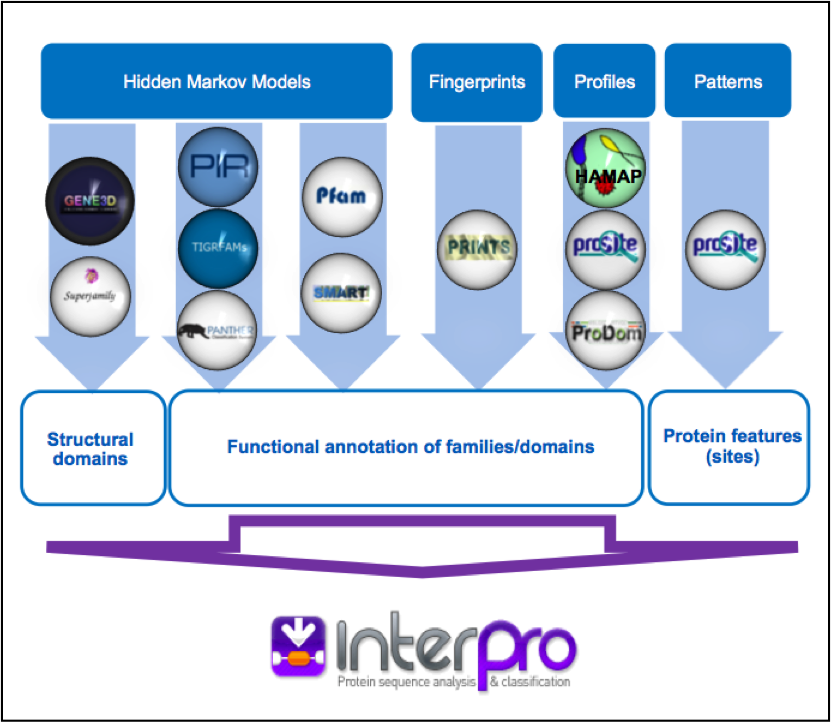
Figure 1. InterPro member databases grouped by the methods, indicated in white coloured text, used to construct their signatures. Their focus of interest is shown in blue text.

Only a subset of the InterPro member databases are used by EMG: Gene3D, TIGRFAMs, Pfam, PRINTS and PROSITE patterns. These databases were selected since, together, they provide both high coverage and offer detailed functional analysis, and have underlying algorithms that can cope with the vast amounts of fragmentary sequence data found in metagenomic datasets.

Assigning functional information to metagenomic sequences

Whilst InterPro matches to metagenomic sequence sets are informative in their own right, EMG offers an additional type of analysis in the form of Gene Ontology (GO) terms. The Gene Ontology is made up of 3 structured controlled vocabularies that describe gene products in terms of their associated biological processes, cellular components and molecular functions in a species-independent manner. By using GO terms, scientists working on different species or using different databases can compare datasets, since they have a precisely defined name and meaning for a particular concept. Terms in the Gene Ontology are ordered into hierarchies, with less specific terms towards the top and more specific terms towards the bottom (see Figure 2).

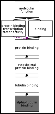Figure 2. An example of GO terms organised into a hierarchy, with terms becoming less specific as the hierarchy is ascended (e.g., alpha-tubulin binding is a type of cytoskeletal binding, which is a type of protein binding). Note that a GO term can have more than one parent term. The Gene Ontology also allows for different types of relationships between terms (such as ‘has part of’ or ‘regulates’). The EMG analysis pipeline only uses the straightforward ‘is a’ relationships.

More information about the GO project can be found http://www.geneontology.org/GO.doc.shtml

As part of the EMG analysis pipeline, GO terms for molecular function,biological process and cellular component are associated to pCDS in a sample via the InterPro2GO mapping service. This works as follows: InterPro entries are given GO terms by curators if the terms can be accurately applied to all of the proteins matching that entry. Sequences searched against InterPro are then associated with GO terms by virtue of the entries they match - a protein that matches one InterPro entry with the GO term ‘kinase activity’ and another InterPro entry with the GO term ‘zinc ion binding’ will be annotated with both GO terms.

Finding functional information about samples on the EMG website

Functional analysis of samples within projects on the EMG website www.ebi.ac.uk/metagenomics/ can be accessed by clicking on the Functional Analysis tab found toward the top of any sample page (see Figure 3 below).

Figure 3. A Functional analysis tab can be found towards the top of each run page

Clicking on this tab brings up a page displaying sequence features (the number of reads with pCDS, the number of pCDS with InterPro matches, etc), InterPro match information and GO term annotation for the sample, as shown in Figure 4 and 5 below.

InterPro match information for the predicted coding sequences in the sample is shown. The number of InterPro matches are displayed graphically, and as a table that has a text search facility.

Figure 4. Functional analysis of metagenomics data, as shown on the EMG website.

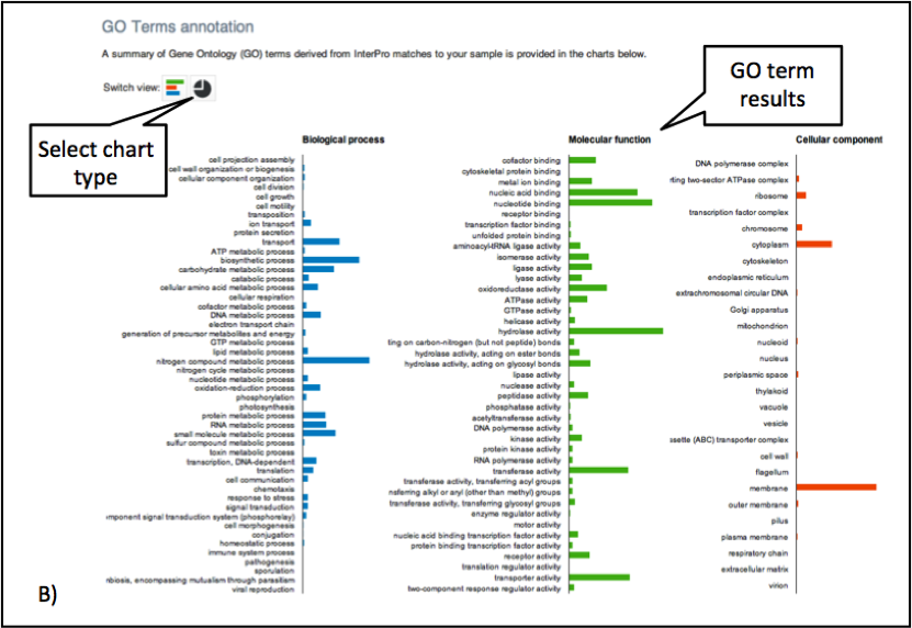Figure 5. The GO terms predicted for the sample are displayed. Different graphical representations are available, and can be selected by clicking on the ‘Switch view’ icons.

The Gene Ontology terms displayed graphically on the web site have been ‘slimmed’ with a special GO slim developed for metagenomic data sets. GO slims are cut-down versions of the Gene Ontology, containing a subset of the terms in the whole GO. They give a broad overview of the ontology content without the detail of the specific fine-grained terms.

The full data sets used to generate both the InterPro and GO overview charts, along with a host of additional data (processed reads, pCDS, reads encoding 16S rRNAs, taxonomic analyses, etc) can be downloaded for further analysis by clicking the Download tab, found towards the top of the page (see Figure 6).

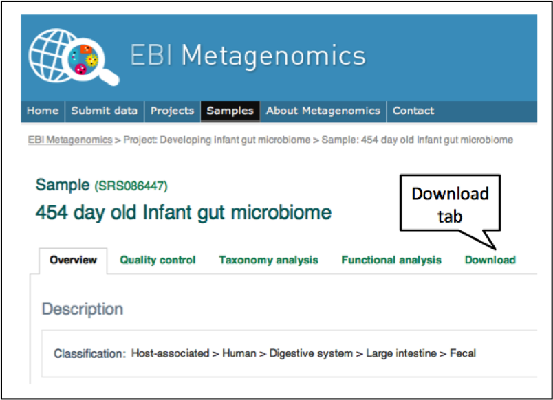Figure 6. Each sample has a download tab, where the full set of sequences, analyses, summaries and raw data can be downloaded.

Practical

---

Browsing analysed data via the EMG website

For this session, we are going to look at the Ocean Sampling Day (OSD) 2014 project, which involved simultaneously sampling from geographically diverse oceanographic sites on Solstice 2014. A map of all of the sampling sites is shown on the project page: https://www.ebi.ac.uk/metagenomics/projects/ERP009703

To get the OSD project page, either follow the above link or open the Metagenomics Portal home page (https://www.ebi.ac.uk/metagenomics/).

1. enter ‘OSD’ in the search box on the top right hand side of the page, and follow the link to project ERP009703. You should now have a Project overview page, which describes the project, submitter contact details, and links to the samples and runs that the project contains.
2. Scroll down to Associated Runs and use the ‘Filter’ search box to find the OSD80_2014-06-21_0m_NPL022 sample (ERS667582).
3. Click on the Sample Name link (not the Run link) to arrive at the overview page, describing various contextual data, such as the geographic location from which the material was isolated, its collection date, and so on.

Question 1:

What is the latitude, longitude and depth at which the sample was collected?

Question 2:

What geographic location does this correspond to?

Question 3:

What environmental ontology (ENVO) identifer and name has the sample material been annotated with?

Now scroll down to the ‘Associated runs’ section of the page. Some samples can have a number of sequencing runs associated with them (for example, corresponding to 16S rRNA amplicon analyses and WGS analyses performed on the same sample). In this case, there is only 1 associated run: ERR770971. Click on the Run ID to go to the Run page.

This page has a number of tabs towards the top (Overview, Quality control, Taxonomy analysis, Functional analysis, and Download). Click on the ‘Download’ tab. Click the file labelled ‘Predicted CDS’ link to save this file to your computer. Find the file (it should be in your Downloads folder), unzip it and examine it using ‘less’ by typing the following commands in a terminal window:

Click on the ‘Download’ tab. Right click the file labelled ‘Predicted CDS (FASTA)’ link, and save this file to your desktop. Find the file, and either double click on it to open it, or examine it using ‘less’ by typing the following commands in a terminal window:

cd ~/Downloads
gzip –d ERR770971_MERGED_FASTQ_pCDS.faa.gz 
less ERR770971_MERGED_FASTQ_pCDS.faa

Have a look at one or two of the many sequences it contains.

You can count the total number of sequences in the file by grepping the number of header lines that start with “>”

grep -c "^> "ERR770971_MERGED_FASTQ_pCDS.faa

In a moment, we will look at the analysis results for this entire batch of sequences, displayed on the EMG website. First, we will attempt to analyse just one of the predicted coding sequences using InterPro (the analysis results on the EMG website summarise these kind of results for hundreds of thousands of sequences).

In a new tab or window, open your web browser and navigate to http://www.ebi.ac.uk/interpro/. Copy and paste the following sequence into the text box on the InterPro home page where it says ‘Analyse your sequence’:

>HWI-M02024:110:000000000-A8H0K:1:1101:23198:21331-1:N:0:TCAGAGAC_1_267
HLLSYRYAYGKFSSTHEATIGGCFLTKDEELDDHIVKYEIWDTAGKNGTIHLPRCTTSKAYXIQVTWYRNAIAAVVVFDVTSRDSFEK

Press Search and wait for your results. Your sequence will be run through the InterProScan analysis software, which attempts to match it against all of the different signatures in the InterProScan database.

Question 4:

Which protein family does InterProScan predict your sequence belongs to, and what GO terms are predicted to describe its function?

Clicking on the InterPro entry name or IPR accession number will take you to the InterPro entry page for your result, where more information can be found.

Return to the overview page for ERR770971.

Now we are going to look at the functional analysis results for all of the pCDS in the sample. First, we will find the number of sequences that made it through to the functional analysis section of the pipeline.

Click on the Quality control tab. This page displays a series of charts, showing how many sequences passed each quality control step, how many reads were left after clustering, and so on.

Question 5:

After all of the quality filtering steps are complete, how many reads were submitted for analysis by the pipeline?

Next, we will look at the results of the functional predictions for the pCDS. These can be found under the Functional analysis tab.

Click on the Functional analysis tab and examine the InterPro match section. The top part of this page shows a sequence feature summary, showing the number of reads with predicted coding sequences (pCDS), the number of pCDS with InterPro matches, etc.

Question 6:

How many predicted coding sequences (pCDS) are in the run?

Question 7:

How many pCDS have InterProScan hits?

Scroll down the page to the InterPro match summary section

Question 8:

How many different InterPro entries were matched by the pCDS?

Question 9:

Why is this figure different to the number of pCDS that have InterProScan hits?

Next we will examine the GO terms predicted by InterPro for the pCDS in the sample.

Scroll down to the GO term annotation section of the page and examine the 3 bar charts, which correspond to the 3 different components of the Gene Ontology.

Question 10:

What are the top 3 biological process terms predicted for the pCDS from the sample?

Selecting the pie chart representation of GO terms makes it easier to visualise the data to find the answer.

Now we will look at the taxonomic analysis for this run.

Click on the Taxonomy Analysis tab and examine the phylum composition graph and table.

Question 11:

How many of the WGS reads are predicted to encode 16S rRNAs?

Question 12:

What are the top 3 phyla in the run, according to 16S rRNA analysis?

Select the Krona chart view of the data icon. This brings up an interactive chart that can be used to analyse data at different taxonomic ranks.

Question 13:

What is the proportion of Polaribacter in the population?

Note

If the cyanobacteria section of the chart looks strange, this is because the version of GreenGenes used for analysis lists chloroplastic organisms under the cyanobacteria category; some of the cyanobacterial counts are, in fact, derived from photosynthetic eukaryotic organisms.

Now we will compare these analyses with those for a sample taken at 2 m depth from the same geographical location.

In a new tab or window, find and open the Ocean Sampling Day (OSD) 2014 project page again. Find the sample OSD80_2014-06-21_2m_NPL022 and examine metadata on the Overview page.

Question 14:

Other than sampling depth, what are the differences between this sample and OSD80_2014-06-21_0m_NPL02?

Scroll to the Assocated runs section, and click on ERR770970. Open the Functional analysis tab and examine the Sequence feature and InterPro match summary information for this run.

Question 15:

How many pCDS were in this run?

Question 16:

How many of the pCDSs have an InterPro match?

Question 17:

How many different InterPro entries are matched by this run?

Question 18:

Are these figures broadly comparable to those for the previous sample?

Now we are going to look at the differences in slimmed GO terms between the 2 runs. There are to ways to do this. First, you can simply scroll to the bottom of the page and examine the GO term annotation (note - selecting the bar chart representation of GO terms makes it easier to compare different data sets). Alternatively, you can use the comparison tool, which allows direct comparison of runs within a project. The tool can be accessed by clicking on the ‘Comparison Tool’ tab, illustrated in Figure 6 below. At present, the tool only compares slimmed GO terms, but will be expanded to cover full GO terms, InterPro annotations, and taxonomic profiles as development of the site continues.

Click on the Comparison tool tab and choose the Ocean Sampling Day (OSD) 2014 project from the sample list and select the OSD80_2014-06- 21_0m_NPL022 - ERR770971 and OSD80_2014-06-21_2m_NPL022 - ERR770970.

Question 19:

Are there visible differences between the GO terms for these runs. Could there be any biological explanation for this?

Navigate back and open the taxonomic analysis results tab for each run.

Question 20:

How does the taxonomic composition differ between runs? Are any trends in the data consistent with your answer to question 19?

Visualising taxonomic data using MEGAN

Next, we are going to look at the taxonomic predictions for all of the runs. To do this, we are going to load them into MEGAN. MEGAN is a tool suite that provides metagenomic data analysis and visualization. We are going to use only a small subset of its features, relating to taxonomic comparison. Detailed information on MEGAN and the analyses and visualisations it offers can be found here:

http://ab.inf.uni-tuebingen.de/data/software/megan5/download/manual.pdf

MEGAN can be downloaded from

http://ab.inf.uni-tuebingen.de/software/megan6/

(there are 2 editions Community and Ultimate. The Community edition is open source and free to download. We will use this version for the tutorial). However, it should already be installed on your Desktop.

Click on the MEGAN icon on your desktop to load the s/w.

We now need to download the full taxonomic predictions for all of the runs in the Ocean Sampling Day project.

Navigate to the Project: Ocean Sampling Day (OSD) page, using the breadcrumb URL link at the top of the page. Click on the Analysis summary tab, which will take you to a set of tab separated result matrix files, summarising the taxonomic and functional observations for all runs in the project.

Click on the Taxonomic assignments (TSV) link, which will download the corresponding file to your computer. When prompted, choose to save the file in the Downloads folder.

Open the Terminal, navigate to the Downloads directory and take a look at the file you have just downloaded (hit q to exit less):

cd ~/Downloads
less -S ERP009703_taxonomy_abundances_v2.0.tsv

You will see it is a large matrix file, with abundance counts for each taxonomic lineage for each run in the project. From the MEGAN menu, choose ‘File’ and ‘Import’. Select ‘CSV Import’ and then find the file you have just downloaded and edited.

From the pop up menu, go with the default options in the Format and Separator sections (which should have the ‘Class, Count’ option selected under format, and the separator set as ‘Tab’) and select ‘Taxonomy’ in classification section, then press ‘Apply’.

There are many different visualisations and comparisons that can be performed using MEGAN, so feel free to explore the data using the tool.

Click on the ‘Show chart’ icon and choose ‘Stacked Bar Chart’. This should give you a bar chart, showing the abundance reads for taxonomic lineages across all of the sampling sites.

Question 21:

Are the number of classified 16S reads roughly equivalent across all of the different sampling sites?

Question 22:

Which run appears particularly enriched in Polaribacter?

You can change between abundance counts and relative abundance using the Options drop menu and choosing % Percentage Scale or Linear Scale.

Change the chart view to ‘Bubble Chart’. This visualisation can be useful when comparing a large number of samples.

Question 23:

Do any samples contain taxa not found in other samples?

Take a look at the Schlegelella genus.

Question 24:

Can you discern any patterns in the geographical distribution of certain species (for example, the cluster of samples enriched for the lactobacillus genus compared to other samples)?

We are now going to take a look at which other datasets in EBI Metagenomics that lactobacilli are found in. Point your browser at https://www.ebi.ac.uk/metagenomics/search/

This interface allows you to search the project, sample and run related metadata and analysis results for all of the publicly available datasets in the EBI Metagenomics resource.

Click on the ‘Runs’ tab. You should now see a number of run-related metadata search facets on the left hand side of the page, including ‘Organism’. Click on the ‘More…’ option under Organism, scroll down to ‘Lactobacillus’ in the pop-up window and select the check box next to it. Now click ‘Filter’. The results page should now show all of the runs that have taxonomic matches to lactobacilli in their datasets. The ‘Biome’ facet on the left hand side of the page now shows the number of matching datasets in each biome category (to save space, the 10 biome categories with the most matching datasets are shown by default).

Question 25:

Which biome category has the most datasets that contain lactobacilli?

Question 26:

How well does this correlate with what’s known about these bacteria?

Finally, we will try to use the interface to find functional proteins present under certain environmental conditions. For example, InterPro entry IPR001087 represents a domain found in GDSL esterases and lipases, which are hydrolytic enzymes with multifunctional properties.

Question 27:

Using the search interface, can you identify the metagenomics datasets sampled from ocean sites at between 10 and 15 degrees C that contain these enzymes?

Question 28:

Can you envisage ways in which this kind of search functionality could be used for target / enzyme discovery?